Version is available at: Dropbox\Download\DM-Xray\dm-xray-setup-ver-1.0.0.1-alpha45x64-prot-signed.exe

What's new?

• In this version we fixed the problem of large dimension voxel data processing
• For cases of data simplification with windows, we added the creation of a model with simplification without windows in order to select a model with the best representation of all cavities.

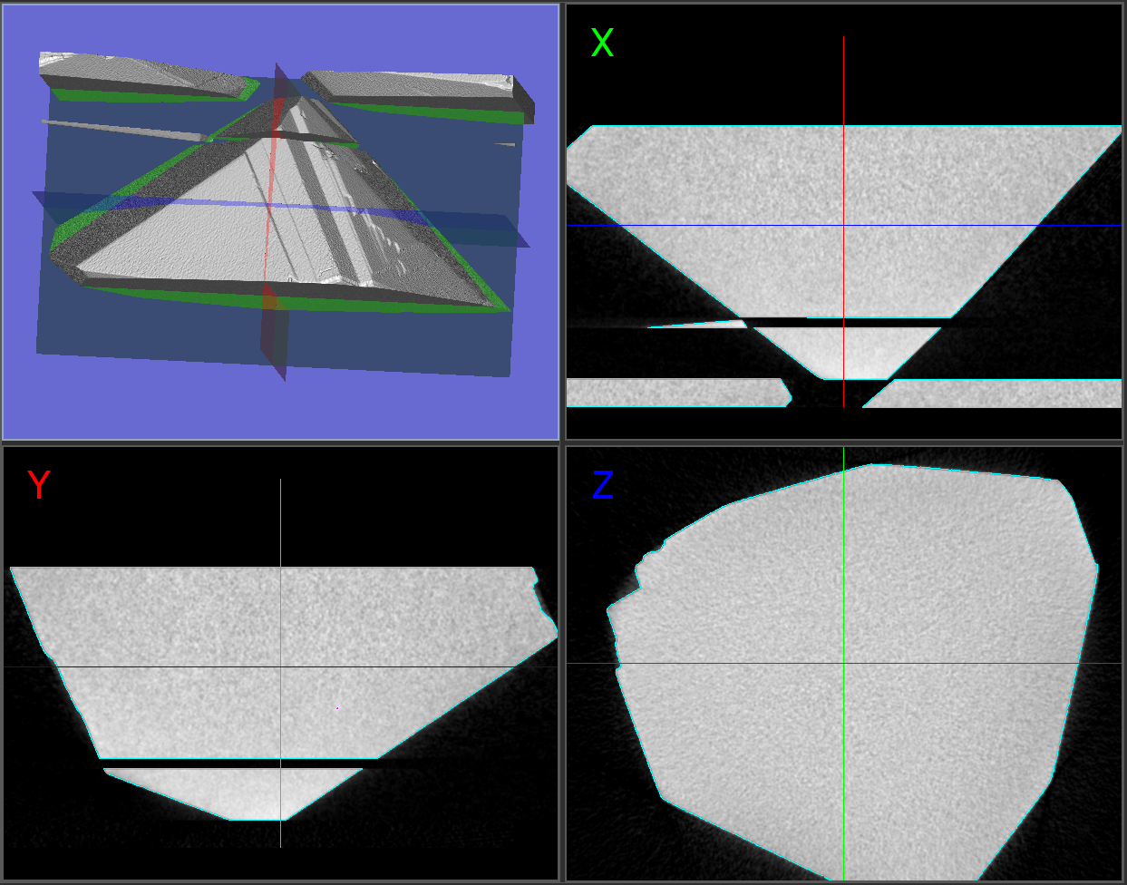
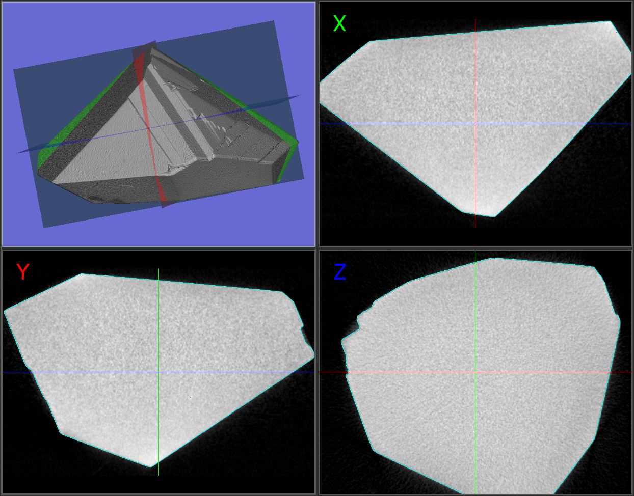
Fixes of processing of voxel data of large dimensions

Comparison of the resulting models

In the DM-Xray, you can get 2 types of models with and without windows. Models obtained with windows give greater accuracy in constructing flat faces, which gives solutions with larger mass (about 0.5%). But these models still have 2 drawbacks. First, there some situations when we can miss small cavity in model with windows. The second drawback is a big time for reconstruction compared to obtaining models without windows (4-5 times bigger). In future releases, we plan to get rid of both flaws. In this release, we offer a solution with obtaining both types of models with and without windows in one algorithm launch and then choose the best model from these two.

For various scenarios of work, the following conventions for naming models are adopted:

• windowless simplification scenario:  "project name_simplified_xx_mic_xxxx_bones";
  
• general simplification with windows: "project name_simplified_with_wins_xx_mic_xxxx_bones";
• convex simplification with windows: "project name_with_cavities_convex_xxxx_bones".

To select the model that most accurately represents all cavities, you can use the following methods:

• Side-by-side models comparison
• Comparing models with the Comparison tool

Side-by-side models comparison

In the left pane representing the simplification results (Services), select the first polygonal model of interest. Usually the shortest name is voxel cube project.

Open any simplified model  by double clicking by name in Service panel. See opened convex model in new tab below.

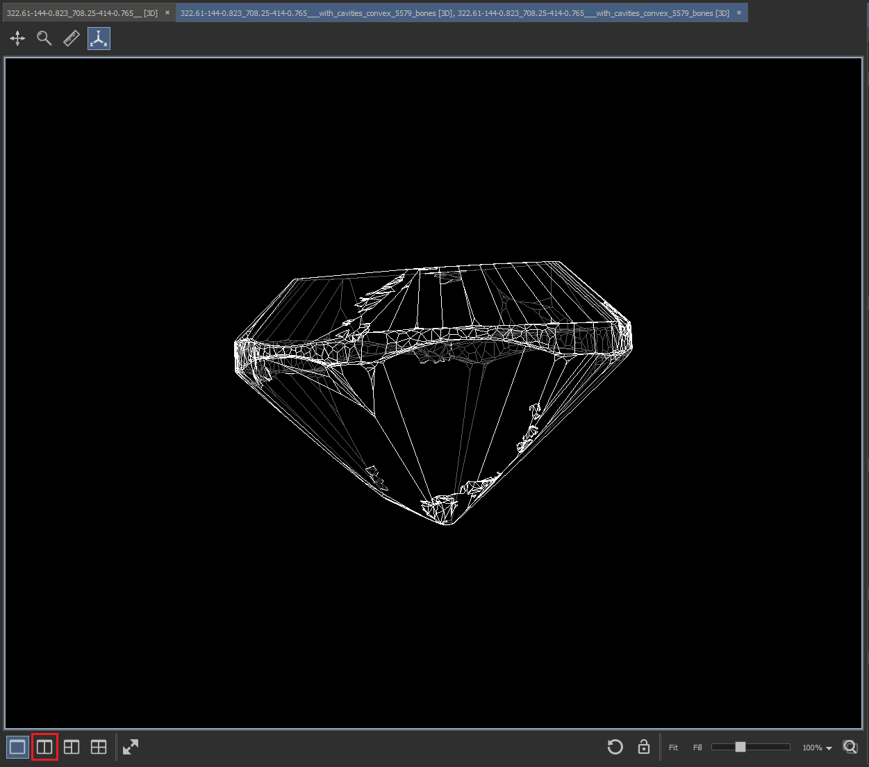
Change view mode to "Two view" by clicking to button .

Than drag and drop another simplified model (unselected with white font color) to empty view:

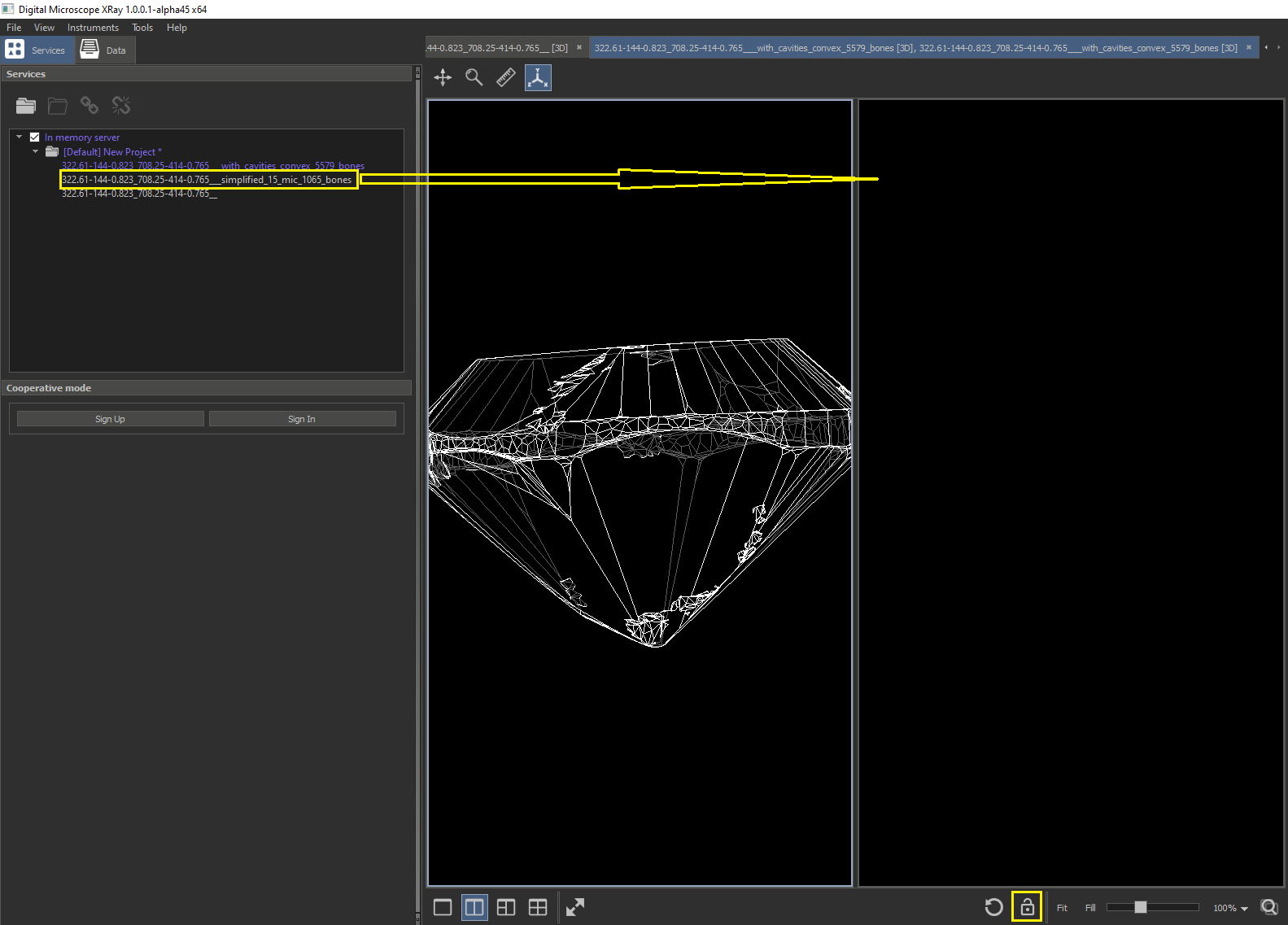
Press  button  in bottom tool panel to synchronize views zoom and pan.

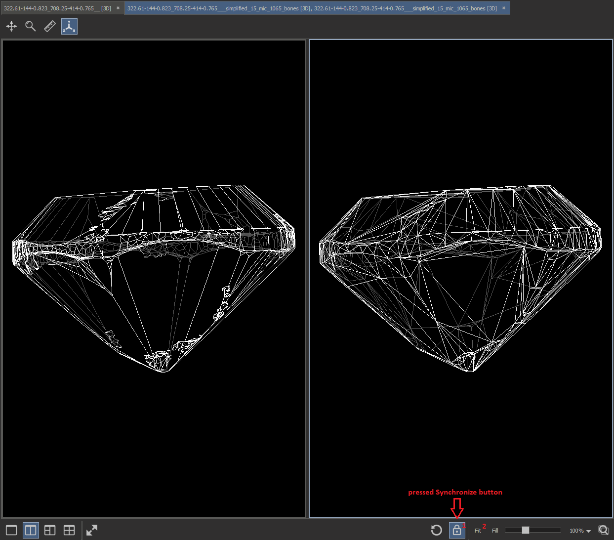
Click the Fit (2) button to scale the models to fit in the 2 views. Rotate any models and compare in synchronize mode.

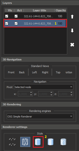
Models can be compared for convenience in another rendering mode, for example, Flat.

To do this, select the bottom layer (1) for each model and set the desired mode (2).

Below 2 synchronized models Flat rendering mode:

After choosing the best model, you can close the previously opened Tabs and reopen the specific model and save.

Comparing Models with the Comparison tool

This comparison method allows you to estimate the difference between models more accurately.

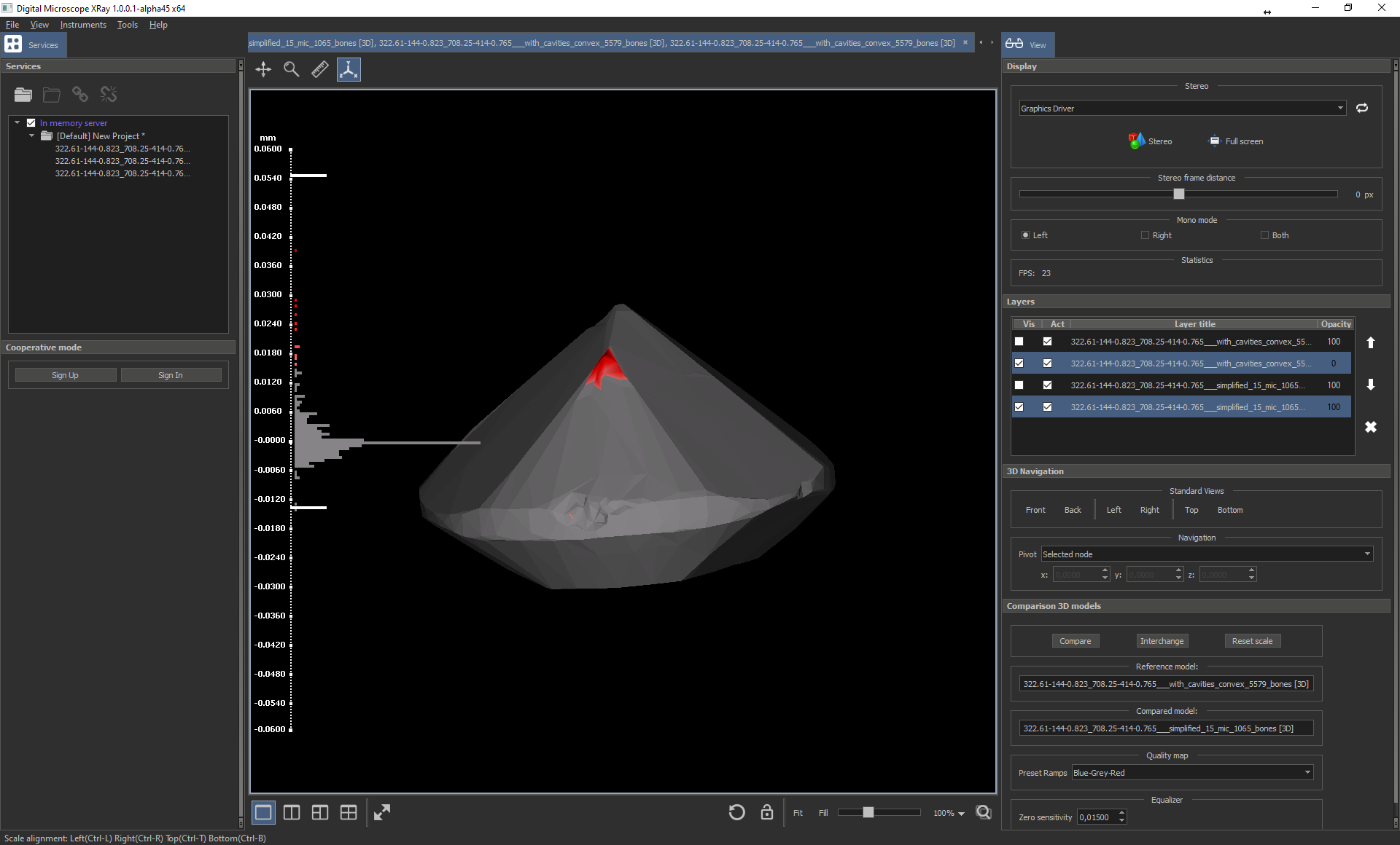
You can find the Comparison instrument after opening  two 3D models in single view (layer) and than simultaneously select two layers in the similarly named panel.

To compare models, not inclusions, you should select even layers (2 and 4).

On figure below you can see in rectangle area №1 two selected layers, and in area №2 "Comparison 3D models".

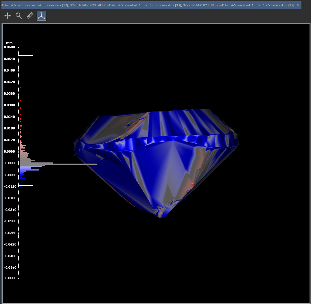
The comparison instrument computes the signed (per vertex) distance between a mesh and a reference mesh. In the box named "Compared model" there is the mesh that is measured, vertex by vertex, computing distance from the Reference model (mesh). You can change the compared model pressing the button "Interchange". To obtain the result of comparison you should press the button "Compare". On next image you can see main view with visualization of comparison result.

To ignore unimportant divergence (close to a zero) you can specify threshold in "Zero sensitivity" spin box.

Set the Zero sensitivity to be equal to the simplification precision (15 mic in this example).

Every divergence value maps into the colour chart. On the Figure below you can see "Blue-Grey-Red" colour chart for the Compared model. For example, values less 15 microns maps into grey colour, 0.024 mm into red, -0.024 mm into blue.

After interchanging you can see the opposite comparison. To find out the difference between the models at a specific point, right-click on the place of interest. See the example below

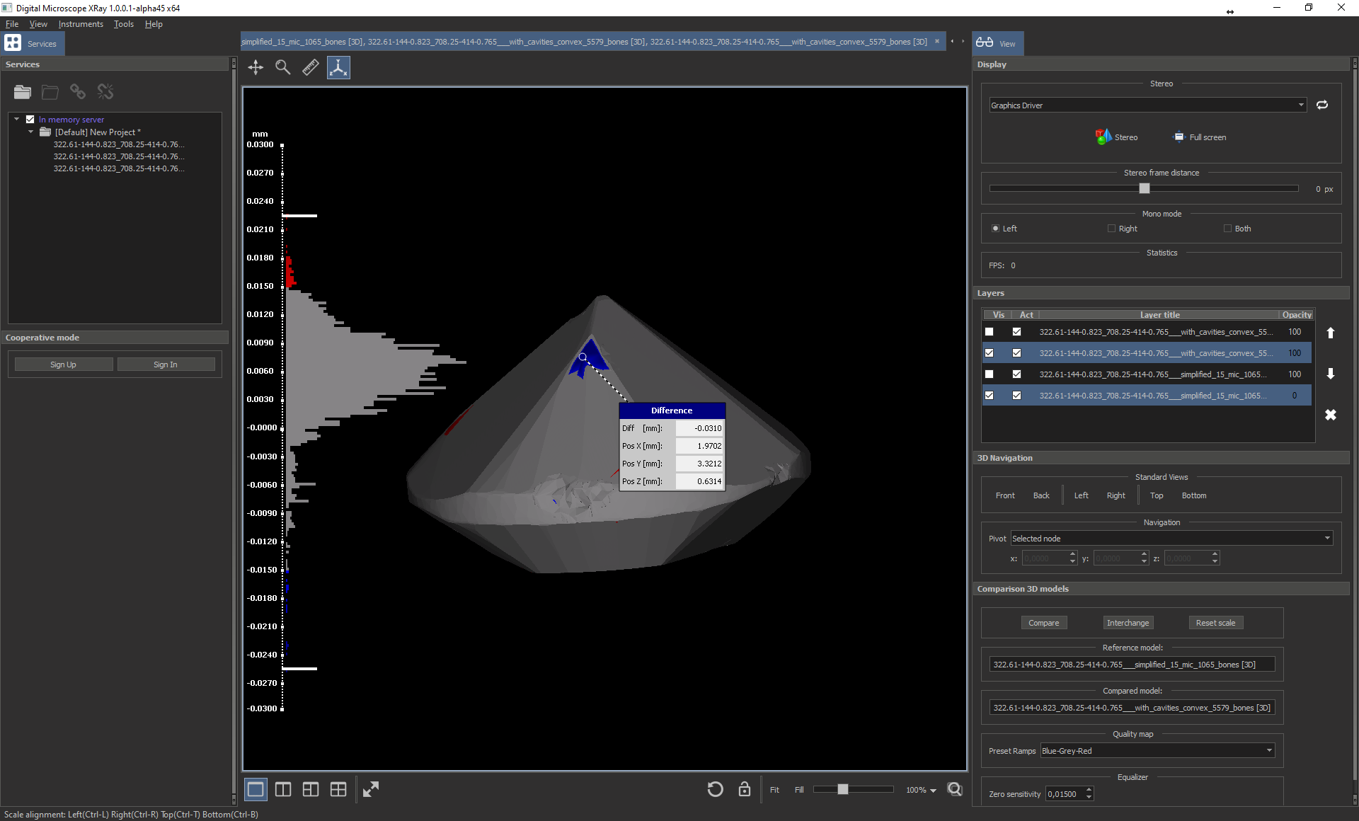
For more details, see the Octonus Stereo Viewer documentation.

Below are the models described in the document:

• 322.61-144-0.823_708.25-414-0.765_simplified_15_mic_1065_bones.dmx (model without windows);
• 322.61-144-0.823_708.25-414-0.765_with_cavities_convex_5579_bones.dmx (model with windows).